Fundamentals of LoRA and low‑rank fine-tuning

1. Introduction1. Introduction

It’s easy to understand why we resort to parameter-efficient fine-tuning of LLMs: fully training them is an extremely costly process.

However, it turns out that a strong pre-trained model doesn’t require many parameters to be adapted for a specific task! This was known as early as 2020 when the authors of Intrinsic Dimensionality Explains the Effectiveness of Language Model Fine-Tuning ran several experiments with encoder-only models of the BERT and RoBERTa classes to explore the 'intrinsic dimensions' of various problems.

Specifically, they analyzed several tasks, and for each, they determined $d_{90}$: the minimum dimension $d$ for which fine-tuning in a $d$-dimensional subspace gives more than 90 percent of full fine-tuning quality. Like this:

The dashed line represents the $d_{90}$ value, and you can see that in many cases, it can be achieved with a $d$ significantly smaller than $D$. Note, by the way, that the horizontal axis is logarithmic.

As LLMs matured, several low-parameter fine-tuning techniques emerged, and the most influential of them is LoRA — the abbreviation comes from low-rank adaptation.

In this long read, we will discuss LoRA and some of its modifications. Namely, I will share with you:

• What is rank from a math point of view, and how to wrap your intuition around it.
• What exactly we mean by fine-tuning a model in a low-dimensional subspace.
• Why LoRA updates come in a two-matrix-product form.
• Which exciting developments arose around LoRA recently.

2. A few words about rank2. A few words about rank

There are many kinds of layers inside LLMs, but in the end their parameters are stored in matrices (luckily, you don’t often encounter tensors in LLMs). And each matrix has a characteristic called rank. Usually, rank is defined like this:

The rank of a matrix $A$ is the maximum number of linearly independent columns (or rows) that can be found in the matrix. (You’ll get the same number if you take rows instead of columns).

While this definition is correct, my experience shows it’s not easy to use. So, let’s consider an equivalent one.

A real matrix $A$ of size $M\times N$ is usually more than just a table filled with numbers; it can represent a variety of algebraic entities. Importantly for our discussion, it can represent a linear transformation $F_A:\mathbb{R}^N\rightarrow\mathbb{R}^M$ mapping from an $N$-dimensional space to an $M$-dimensional space (mind the order!). My favorite way to characterize rank is:

The rank of a matrix $A$ is $\dim{\mathrm{Im}(F_A)}$, the dimension of the image of $F_A$.

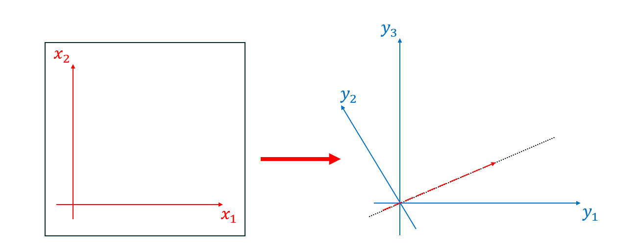
For example, if $A$ is $3\times 2$, it represents a linear transformation $\mathbb{R}^2\rightarrow\mathbb{R}^3$, and its rank could be $2$ (top picture), or $1$ (bottom picture), or even $0$ if the image is zero:

While I won’t formally prove the equivalence of these two definitions here, let me remind you that the columns of a matrix of a linear transformation are precisely the images of the standard basis vectors. Here is an example of a $4\times3$ matrix corresponding to a linear map $\mathbb{R}^3\rightarrow\mathbb{R}^4$:

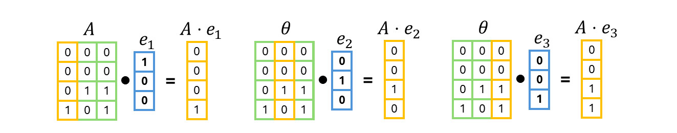
If you need a basis for the image of $F_A$, you can take a maximal linearly independent subset of $A$, such as $Ae_1, Ae_2$. Thus, the rank is $2$.

3. Low-rank adaptation — LoRA3. Low-rank adaptation — LoRA

The essence of LoRA is:

Let’s only do low-rank parameter updates.

To clarify, consider some weight matrix $W$, which is, of course, a matrix of some linear transformation $F_{W}: \mathbb{R}^M\rightarrow\mathbb{R}^N$. A low-dimensional update of $F_{W}$ is a new transformation $G$:

$$G (x) = F_{W}(x) + F'(x),$$

where the image of $F'$ is low-dimensional.

Here is an example where $F_{W}:\mathbb{R}^2\rightarrow\mathbb{R}^3$ and $F'$ has a rank of $1$:

You see that adding $F'$ changes only what happens on the green line.

LoRA suggests the following:

• We freeze $F_{W}$,
• We only fine tune $F'$, and we demand that the rank of its matrix $W'$ is $\leqslant r$, where $r$ is a hyperparameter.

The problem is that optimizing $W'$ over a subset is usually tricky, to say the least. Can we find a convenient parametrization for rank-$\leqslant r$ matrices? It turns out that yes, and for this purpose, we will revisit our dimension-of-the-image description of rank.

4. Parametrizing a low-rank matrix4. Parametrizing a low-rank matrix

Let’s take another look at our rank-1 example:

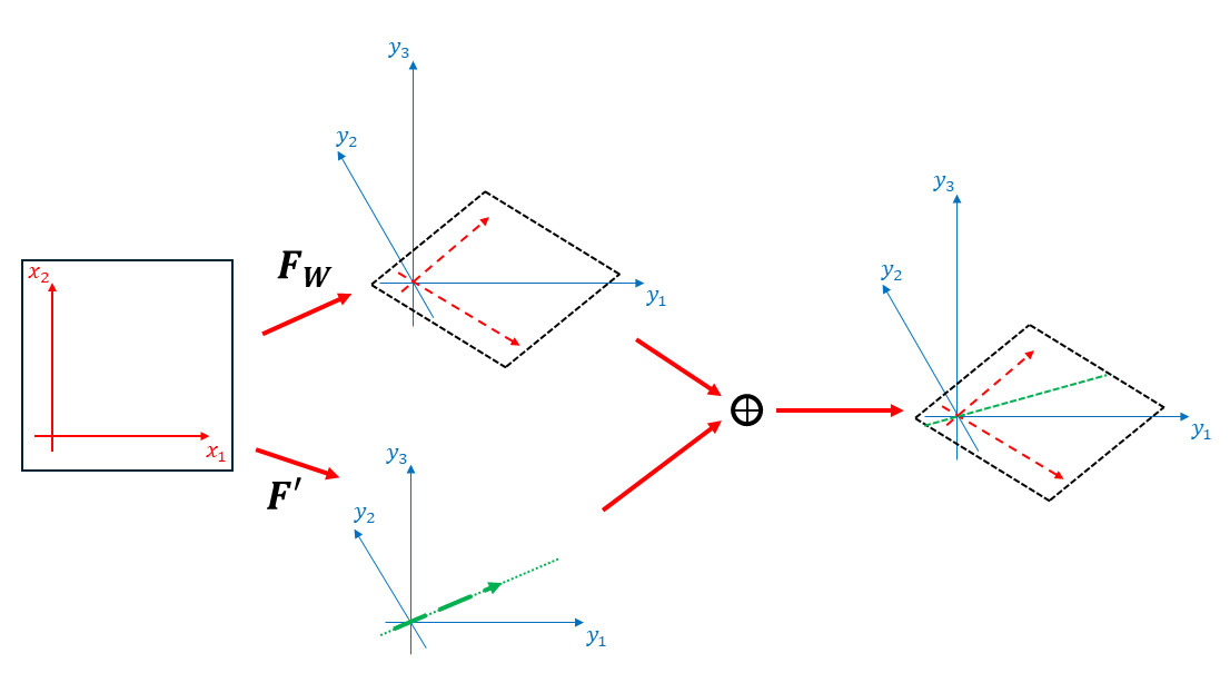
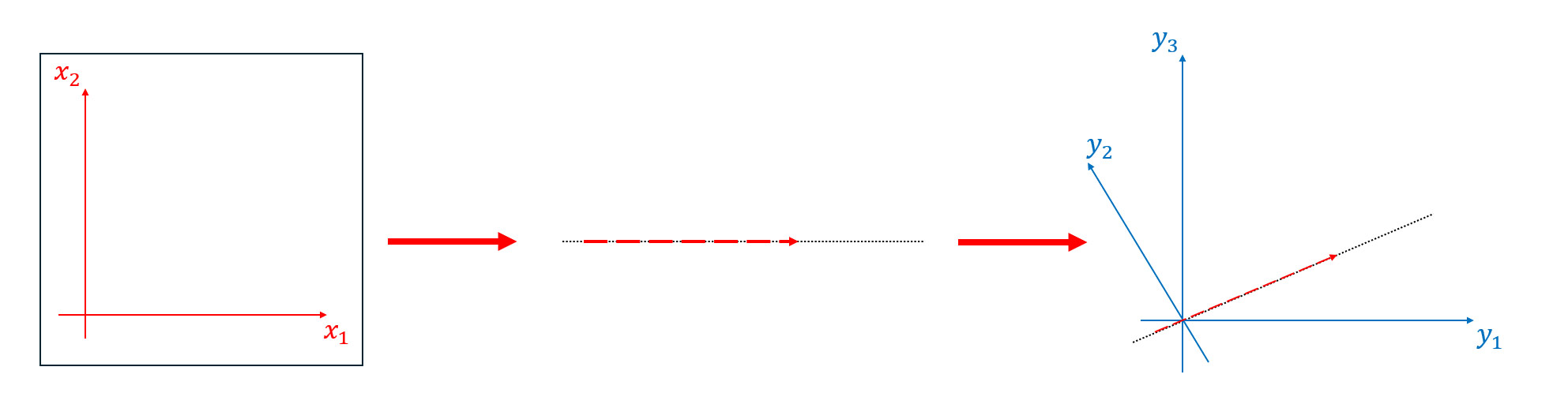
This transformation can be done in two stages:

1. First, we map a 2d plane onto a line using a matrix $A$ of shape $1\times 2$.
2. Then, we embed this line into a 3d space using a matrix $B$ of shape $3\times 1$.

Like this:

Now, we have $F_W (x) = F_B (F_A (x))$ or, in matrix terms:

$$\underset{3\times 2}{W} = \underset{3\times 1}{B}\cdot \underset{1\times 2}{A}.$$

In exactly the same way, we can demonstrate that any $M\times N$ matrix $W$ of rank $r$ can be decomposed as

$$\underset{M\times N}{W} = \underset{M\times r}{B}\cdot \underset{r\times N}{A}.$$

Moreover, if there is a decomposition

$$\underset{M\times N}{W} = \underset{M\times s}{B}\cdot \underset{s\times N}{A},$$

then $\mathrm{rk}{W}\leqslant s$. Note: the rank can be less if the ranks of $A$ and $B$ are less than $s$.

And that’s exactly what we do in LoRA. We decompose $W' = BA$ and train matrices $B$ and $A$ without any additional constraints!

Now, you should better understand what happens in this image (sourced from here):

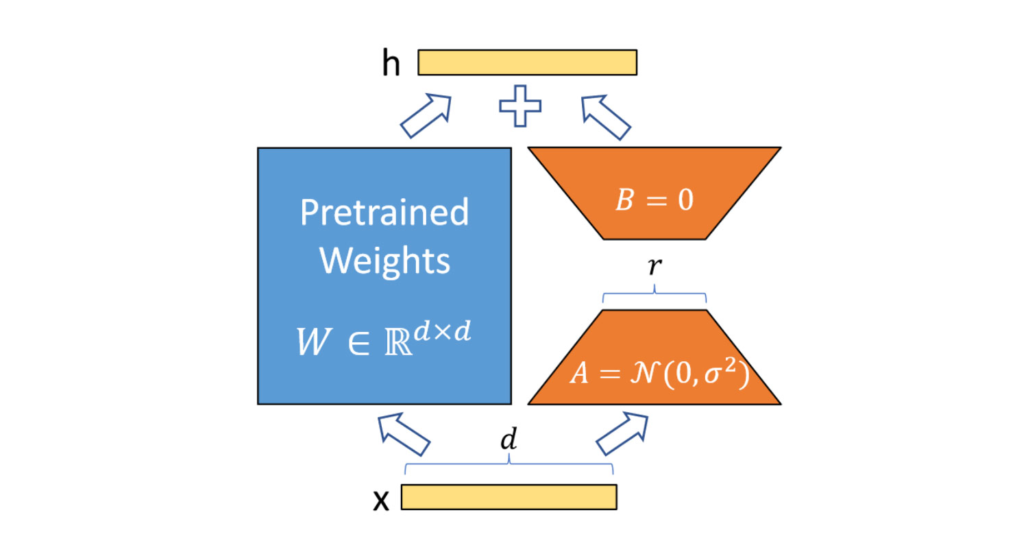
Now, we can explicitly calculate how much additional memory LoRA requires. For example, if the original $W$ was $4096 \times 4096$, like in Mistral’s q_proj layer, and the LoRA rank is $r = 8$, then

• $A$ is of shape $8\times4096$,
• $B$ is of shape $4096\times8$,

giving $8\cdot4096 + 4096\cdot8 = 65,536$ new parameters which is only about $0.4\%$ of the $4096\cdot4096$ parameters of $W$.

There is no general rule, but usually quite small values of $r$ are used. It’s reasonable to go with $8$, or $16$, or, if you’re especially generous, with $64$, although I wouldn’t start with it. Usually, all dense layers, except for the embedding layer, are fine-tuned, that is:

• Query, key and value projections (q_proj, k_proj, v_proj layers) and the output projection of the attention block (o_proj layers),
• All the dense layers inside the Feedforward block.

Often, a dropout layer is also added before $BA$ with $p=0.1$ or likewise small.
The one thing I would add is how we initialize $B$ and $A$. We want to start fine-tuning from the pre-trained weights $W$, so $W'$ should initially be zero. It’s easy to do this by setting the initial $B$ to zero, as depicted in the image above.

LoRA has proven itself a worthy companion for any LLM engineer and a default choice for fine-tuning tasks.

It has been observed, though, that LoRA often yields worse results than full fine-tuning. Of course, we could blame a lack of parameters, but there are additional inefficiencies in LoRA, which we’ll discuss in upcoming sections.

4.1. Intrinsic dimensionality: experiment details4.1. Intrinsic dimensionality: experiment details

I previously mentioned the paper Intrinsic Dimensionality Explains the Effectiveness of Language Model Fine-Tuning, which showcased that certain task can be successfully solved with low dimensional parameter updates. I skipped the details of the experiment setup, so I’ll briefly explain it now.

The LoRA update is expressed as:

$$W \mapsto W + BA,$$

where $F_A$ projects to an $r$-dimensional (low-dimensional) space, and $F_B$ embeds the latter into the image space of $F_W$.

What the authors of the Intrinsic Dimensionality paper did is:

• They took specially structured random $B$ and froze it.
• They then trained $A$.

This means that for each experiment, they fixed a random subspace and trained the updates within it, while LoRA trains both the subspace ($B$) and the updates within it ($A$).

It’s interesting that we can get meaningful results even when making updates in a randomly selected subspace with a random frozen $B$. But of course, it’s much better to make them trainable.

5. PiSSA: using SVD to do updates in a more meaningful subspace5. PiSSA: using SVD to do updates in a more meaningful subspace

When we’re implemetingwe implementdo LoRA, $B$ evolves through stochastic gradient descent, allowing the subspace where the updates occur and, develop randomly. This raises the question: can we identify a 'good' starting subspace?

The answer might be yes. We have a good old method for identifying 'meaningful' subspaces, known as singular value decomposition (SVD). Let’s briefly revisit what it is.

By definition, a singular value decomposition (SVD) of a matrix $W$ is

$$\underset{M\times N}{W} = \underset{M\times M}{U}\cdot\underset{M\times N}{\Sigma}\cdot \underset{N\times N}{V^T},$$

where:

• $U$ is orthogonal, meaning the columns $u_i$ of $U$ are mutually orthogonal vectors of length $1$: $\langle u_i, u_j\rangle = 0$ for $i\ne j$, and $|u_i| = 1$. (The same is true for rows of $U$ because $U$ is square).

• $V$ is also orthogonal.

• $\Sigma = \mathrm{diag}(\sigma_1,\sigma_2,\ldots)$ is diagonal with $\sigma_1 \geqslant \sigma_2 \geqslant \ldots \geqslant 0$. These $\sigma_i$ are known as the singular values of $W$. Just be aware that $\Sigma$ is not always square; for example:

To move on, we need to tinker with matrices a bit. First, we can put $\sigma_i$ into the columns of $U$ and the rows of $V^T$ (which are the transposed columns of $V$):

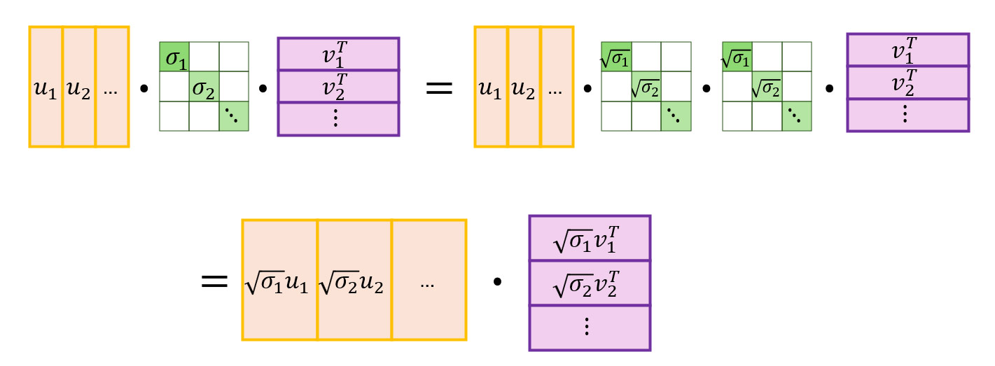
Next, we use the following matrix identity:

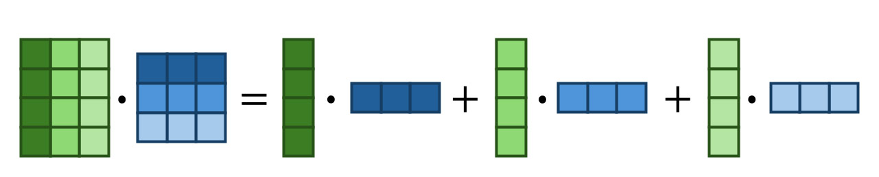
to reformulate SVD as:

Now, let’s recall that $\sigma_1 \geqslant \sigma_2 \geqslant \ldots \geqslant 0$. Moreover, in most real cases, the singular values $\sigma_i$ decline rapidly, enabling us to select a reasonable $r < M, N$ such that $\sigma_{r+1}$ is significantly less than $\sigma_1$. We can then suggest that

• $(\sqrt{\sigma_1}u_1) (\sqrt{\sigma_1}v_1)^T + \ldots + (\sqrt{\sigma_r}u_r) (\sqrt{\sigma_r}v_r)^T$ encapsulates the meaningful components, while
• $(\sqrt{\sigma_{r+1}}u_{r+1}) (\sqrt{\sigma_{r+1}}v_{r+1})^T + (\sqrt{\sigma_{r+2}}u_{r+2}) (\sqrt{\sigma_{r+2}}v_{r+2})^T + \ldots$ represents 'noise'.

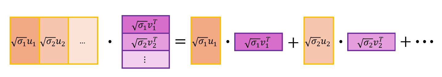
Reapplying the green-and-blue matrix identity, we can depict it this way:

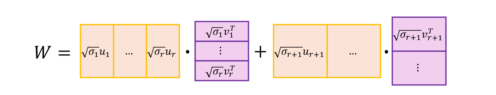
Here, the first part of the sum is meaningful and the second is 'noise'. We can distill this further into:

$$W = {\color{orange}{B}}{\color{magenta}{A}} + W_{\mathrm{noise}}$$

Here’s what we have here:

• The summand ${\color{orange}{B}}{\color{magenta}{A}}$ likely represents the 'important' part of the matrix.
• ${\color{magenta}{A}}$ is a projection to an $r$-dimensional space, while ${\color{orange}{B}}$ embeds this space into the image space of $W$ as the $r$-dimensional subspace $S_r$.

Caution! When using SVD, we persuade ourselves that all the interesting things happen in $S_r$. However, this is not always true. The principal components $(\sqrt{\sigma_1}u_1) (\sqrt{\sigma_1}v_1)^T + \ldots + (\sqrt{\sigma_r}u_r) (\sqrt{\sigma_r}v_r)^T$ are larger but not necessarily more interesting or useful. Sometimes, the finest details are the most important ones. However, SVD may give us a good starting point for training LoRA.

The PiSSA paper suggests exactly that. The authors take

$$W = {\color{orange}{B}}{\color{magenta}{A}} + W_{\mathrm{noise}}$$

as we did earlier and further fine-tune $A$ and $B$. The results are nice; the authors claim to beat LoRA in their experiments, and they also show that PiSSA performs better than QLoRA in a quantization strategy when the base model is set to 'nf4' precision and frozen, while the adapters are trained using 'bfloat16' precision.

6. DoRA: decoupling magnitude and direction updates6. DoRA: decoupling magnitude and direction updates

The authors of DoRA: Weight-Decomposed Low-Rank Adaptation did an insightful analysis of magnitude and direction updates during full fine-tuning versus LoRA.

Consider the columns of the weight matrix

$$W = \left[\begin{matrix}w_1, w_2,\ldots, w_N\end{matrix}\right]$$

As we remember, each $w_i$ is the image under $W$ of the standard basis vector $e_i$. During fine-tuning, the vectors $w_i$ change in both magnitude and direction. It’s curious to see that the patterns of these changes differ between full fine-tuning (FT) and LoRA. Let’s explore how. We decompose the matrix as

$$W = m\odot\frac{W}{||W||},$$

where $m$, also denoted by $||W||$ (magnitudes), is the vector

$$||W|| = \left (||w_1||, ||w_2||, \ldots, ||w_N||\right),$$

$\frac{W}{||W||}$ (directions) is the following matrix:

$$\frac{W}{||W||} = \left[\begin{matrix}\frac1{||w_1||}w_1, \frac1{||w_2||}w_2,\ldots,\frac1{||w_N||}w_N\end{matrix}\right],$$

and $\odot$ stands for a special kind of element-wise product.

Now, here’s an image illustrating the patterns of change:

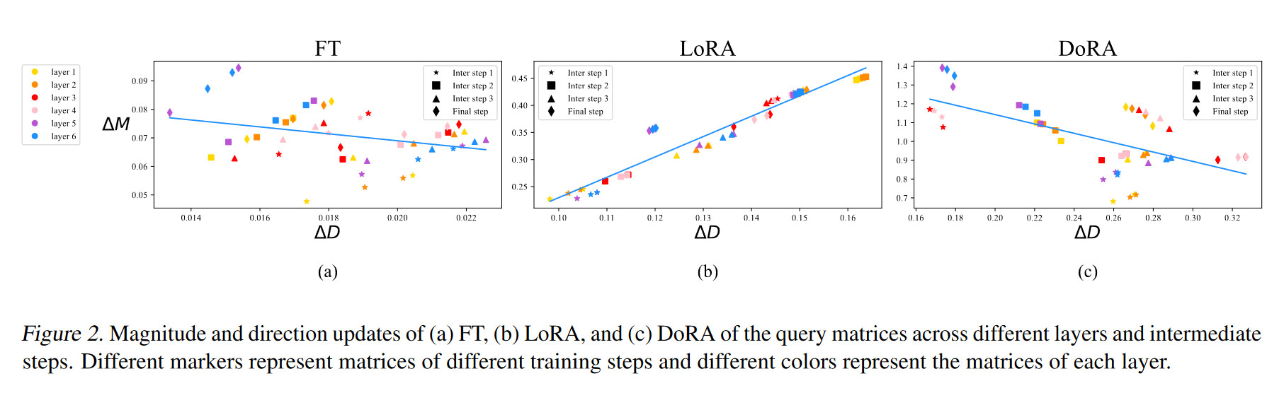
On the $\Delta M$ axis, we have MAE between $||W||$ before and after fine-tuning. On the $\Delta D$ axis, we have mean $(1 — \cos (\cdot, \cdot))$ distance between $\frac1{||w_i||}w_i$ before and after fine-tuning.

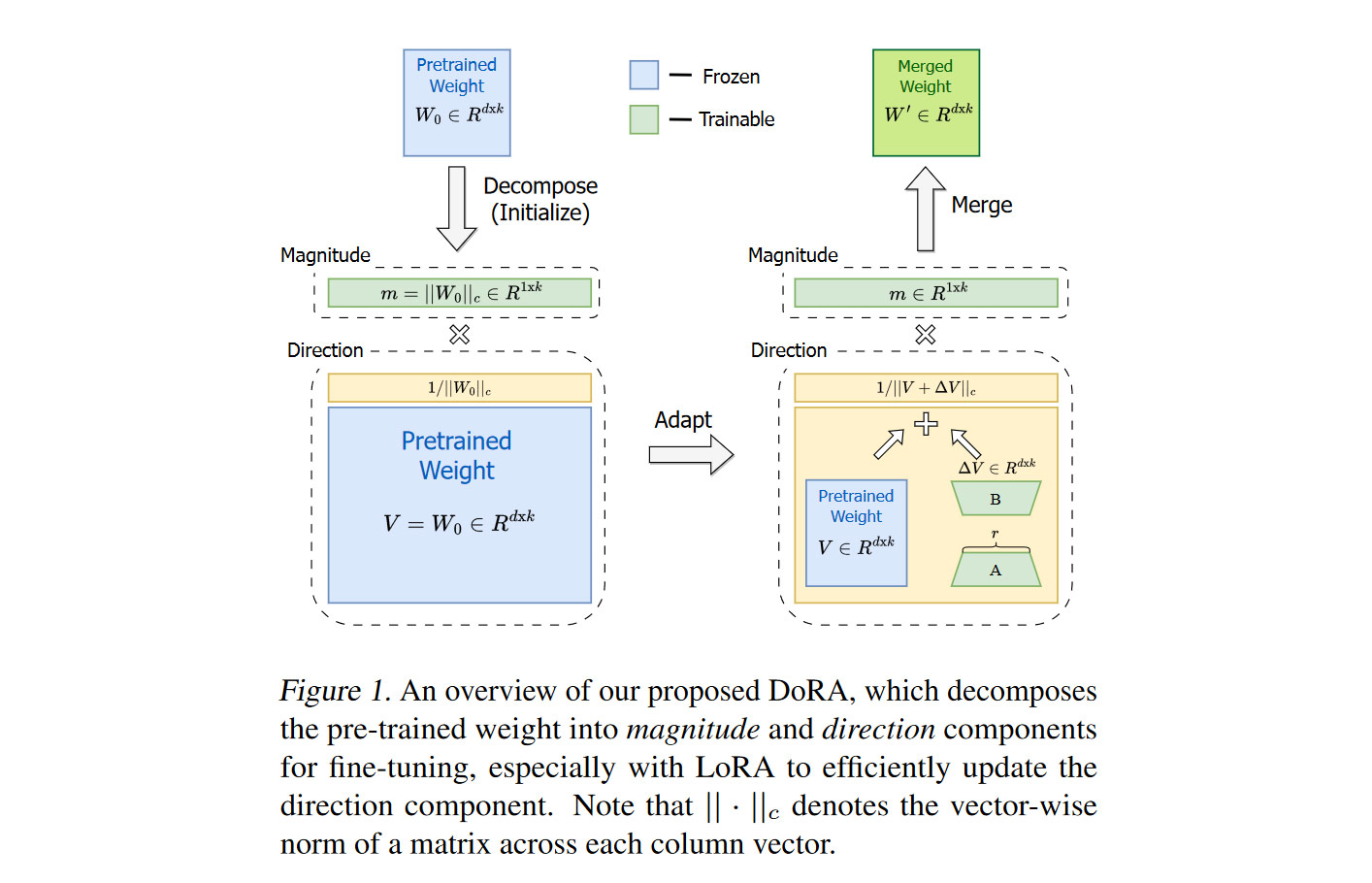
For LoRA, there is a notable positive correlation between $\Delta D$ and $\Delta M$, while for full fine-tuning (FT), these values exhibit a weaker negative correlation. This hints that in LoRA, magnitudes and directions might become entangled in a suboptimal way. To address this, the authors of DORA suggest decoupling them during fine-tuning. Specifically, they update the weight matrix as

$$W' = m \odot \frac{W_0 + BA}{||W_0 + BA||},$$

where:

• $W_0$ is the initial $W$ before fine-tuning,
• $m$ is a trainable magnitude vector, initialized as $||W_0||$,
• $BA$ is a low-rank LoRA summand with trainable matrices $A$ and $B$,
• Division by $||W_0 + BA||$ means division of each column of $W_0 + BA$ by its length.

The method can be summarized in this table:

As you could see in the earlier plots, the correlation between magnitude and direction updates exhibits a weak negative correlation, similar to what we see in full fine-tuning. This correlation can be really important, as in experiments, DORA consistently outperformed LoRA (well, if +1 point in quality is enough for you).

This article was inspired by my experience of teaching linear algebra and by discussions at the paperwatch meetings of the Practical Generative AI course by School of AI and Data Technologies. If you’re interested in studying LLMs and other generative models, their internal workings and applications, check out our program.