
Transformer alternatives in 2024
With this article, we are starting a new category in the blog, the one dedicated to AI research. Expect these posts to be very technical and insightful. The first one is about possible alternatives to the key architecture of modern ML.
1. Introduction
Transformer models are cool, but they do have performance issues. In the classic setup, during the attention phase, each token must “attend” to every other token, leading to quadratic complexity. Moreover, to avoid recalculating all keys and values at each decoding step, they are stored in a key-value cache. These two factors make transformers punishingly expensive for processing long sequences.
There are several intrinsic approaches for addressing these issues. Some focus on making attention less compute-hungry. An example is Group-Query attention that proposes retaining only one attention head for keys and values, thus accelerating attention and reducing the kv-cache size. Others, like FlashAttention, seek to leverage hardware features and algorithmic advancements to make the attention mechanism more efficient without altering its core essence.
However, there is also research focused on entirely eliminating attention and its associated quadratic complexity. To date, the most successful attempts involve Linear (without nonlinearity in the recurrence) RNNs. Why are Linear RNNs advantageous?
- As RNNs, they are efficient at the inference stage: no need to consider the entire previous sequence, only the preceding step.
- Thanks to the absence of nonlinearities, Linear RNNs can be reformulated as convolutions (see 2.3), which, with a mix of math, Fast Fourier Transforms, hardware considerations, and a bit of luck, allows for effective parallelization during training.
- They can be linked to continuous-time state space models, opening up even more possibilities for improvement and analysis.
So far, the pinnacles of this research are Mamba and Griffin. In this long read, you will learn what design choices led to creation of these models.
2. The main story: from RNNs to Mamba and beyond
2.1. Beyond attention: any ideas?
A typical transformer-based LLM architecture looks like this:
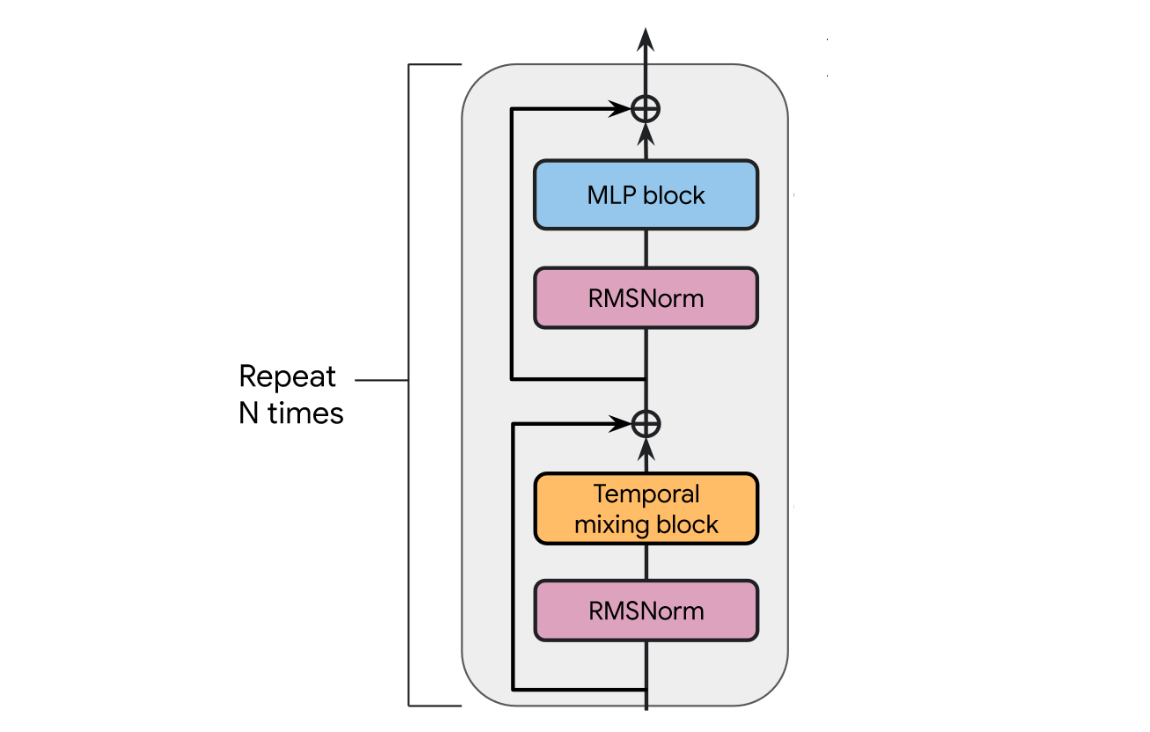
Attention contributes by propagating information across time, unlike the MLP block, which solely performs channel mixing.
We have other mechanisms for temporal propagation, namely:
- Convolutions. They are highly parallelizable, but capturing a long context requires a long kernel, and this will hinder its efficiency: too many trainable parameters in a kernel of a size of a typical transformer kv-cache. So, it is either no gain in comparison to transformers or restricted locality.
- Recurrence. In theory, it allows to capture all the previous context while keeping the complexity linear. However, in practice, information can be lost along the way.
Despite these drawbacks, the ideas behind today’s non-attention-based NLP models stem from different combinations of convolutional and recurrent principles.
And it all starts with a simple but unexpected thing: Linear RNNs are good.
2.2. Linear RNNs are good
The idea that something non-linear must come between linear layers lies in the foundation of deep learning. So, traditional RNNs operate as follows:

where uₜ is the input, yₜ is the output, xₜ is the hidden state, g is a nonlinearity, and Duₜ is a skip-connection. Okay; skip connections were not typical in the mid-2010s, but later on, we have learned to value them. Note that I deliberately omitted the bias terms.
Let’s call Linear RNN a network consisting of several (RNN + MLP) blocks, where g is set to identity in each of the recurrent layers.
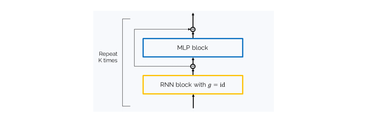
You might scoff at such a network, but the authors of the Resurrecting RNNs paper demonstrate that it is quite expressive and can even be better than networks with tanh or ReLU for g:
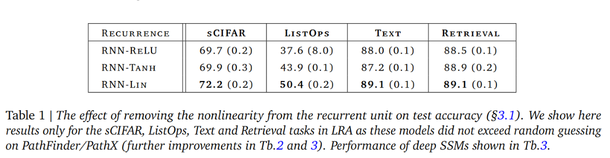
It seems like it is enough to have nonlinearities in the MLP blocks.
2.3. Time-parallel usage: Linear RNNs as convolutions
Let’s consider the full pass of information through a Linear RNN:

for a sequence u₀, u₁, … (where u₀ = 0) this gives

This can be interpreted as a convolution

where L is the potential max length of a sequence, Duₖ works as residue connection, and

is the convolution kernel.
This convolution is parameter-efficient: the number of its trainable parameters does not scale with L. But still, the convolution is very, very long, so we need several hacks to make it work efficiently.
Hack 1. Matrix A should be simple
Often, it is diagonal.
It can be complex diagonal as the Linear Recurrent Unit (LRU) with its intricate parametrization of A = diag (λ) and additional normalization γ: 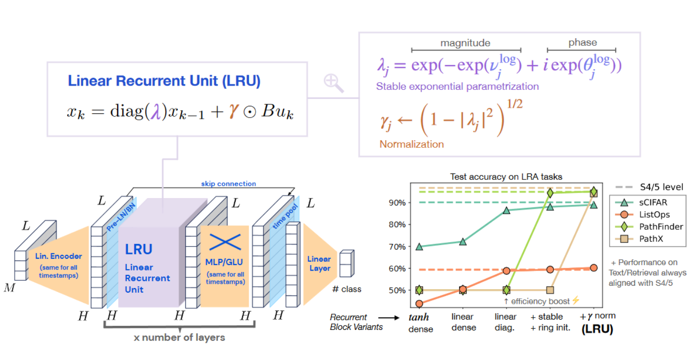
The paper has an elegant mathematical explanation for this parametrization.
It can also be diagonal + low rank or even non-trainable. If a matrix is sufficiently simple (quasiseparable, see here), then the kernel

can be computed in

time and memory for some q, where d is the dimension of the implicit states xₖ. This is at least faster than full attention in a transformer.
I would like to add that the choice of parametrization and/or initialization of A is determined not only by our desire to compute convolutions efficiently. It is also crucial to ensure that a Linear RNN in its recurrent mode captures the previous context well.
Here is a nice way of thinking about it: memorizing ability equals the ability to compress information about the previous context in a vector of a given dimension. Let’s make a step from discrete sequences to functions f (t) of variable t. We know a good way of vectorizing a function: Fourier analysis. A development of this approach allowed the authors of the Hippo paper to come up with an influential way of initializing the matrix A for state space models, a continuous-time version of Linear RNNs, which you’ll encounter quite soon.
Hack 2. You need to know how to speed up a convolution
A must-have improvement is using the convolution theorem

connecting convolution and pointwise multiplication (⊙) via Fast Fourier Transform F. This allows to decrease the complexity of convolution from O(L²) to O(L logL). It is also important to leverage hardware (GPU) specifics.
Convolutional formulation allows for fast parallelized training. However, it is sometimes used at inference stage as well. The models that do it are sometimes referred to as long convolution sequence models (LCSMs). Some papers even use primarily convolutional architectures with special kernels and windows (see, for example, Hyena Hierarchy or Monarch Mixer). In such cases, you may need to do additional work to use a pure-convolutional model in recurrent mode (see Laughing Hyena Distillery).
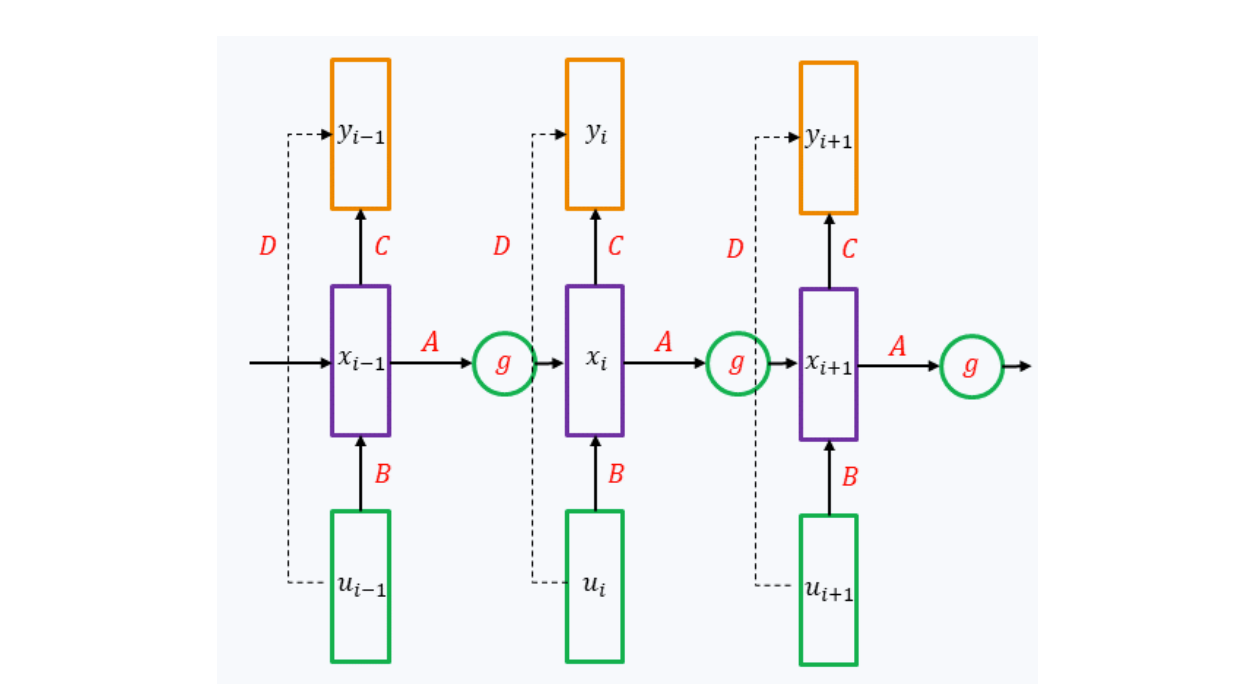
2.4. Continuous-time recurrence: State space models
State space models were initially created in 1960s to model continuous-time processes. A state space model is defined by the following ODE (ordinary differential equation):

where ẋ(t) stands for the time derivative

Note that the role of A in this model differs a lot from the role of A in the recurrent model. However, if we choose a (small) step T and set

we can make a discretization of (1) as

Here,

However, working with matrix exponents is tough, so given that T is small, we can use various approximations for it. The simplest is exp(AT) ≈ I + AT, which gives us approximations referred to as Euler method:

so that

However, bilinear transform is also widely used:

Please keep in mind that even when AI engineers work with discretized versions, they often still parametrize SSMs with A and B from continuous-time formulation.
An important remark about dimensions. All the formulas in this subsection are written for one-dimensional uₜ and one-dimensional yₜ. If u is d-dimensional, the same process occurs for every coordinate of u. This means, in particular, that a state space layer only performs time mixing (different coordinates of uₜ do not influence each other’s outputs) and relies on the MLP layer for channel mixing.
Why does continuous formulation matter? There are several reasons:
- A continuous-time model can be discretized to various resolutions, allowing us to adapt it to different sampling frequencies without retraining.
- Recent approaches make the discretization step data-dependant, thus creating an efficient feature selection technique. Mamba (see 2.6) is known to leverage this.
2.5. Architectures with Linear RNNs
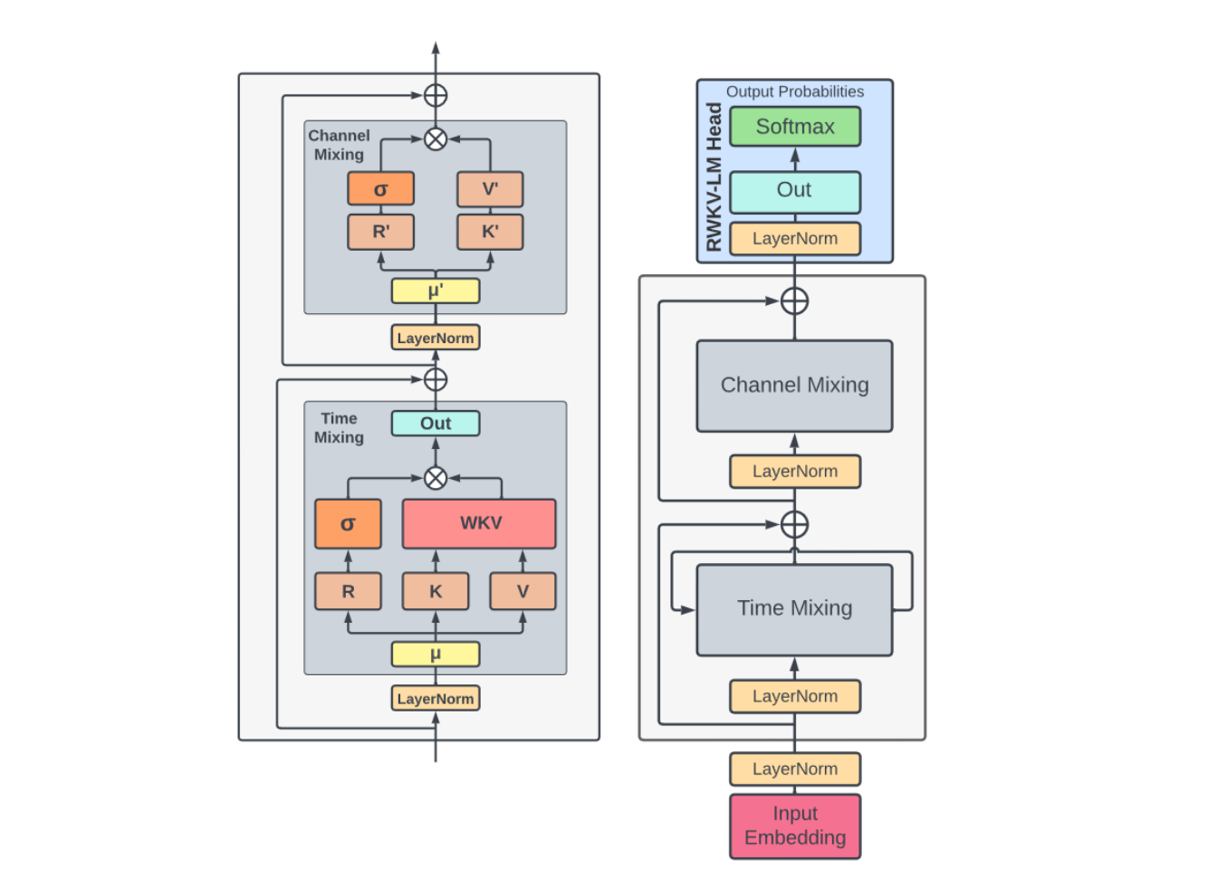
Linear RNNs take the place of an attention mechanism in the LM architectures. Here is an example, RWKV (Receptance Weighted Key Value, with the WKV block being recurrent-based):
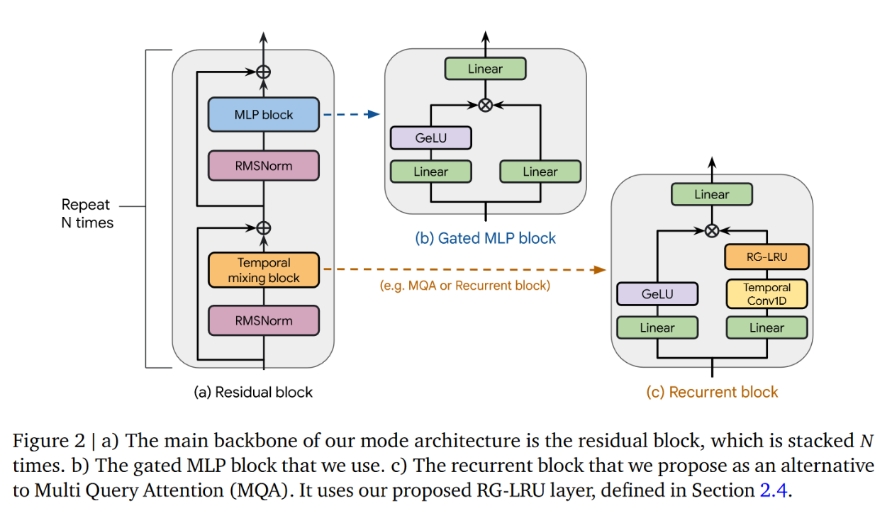
And, finally, Hawk:
Note that 1D convolutions also appear a way of establishing local connectivity in the time domain.
2.6. Data-dependent gating
Before 2017, when RNNs were still state-of-the-art in NLP, they used a complex gating mechanism to control memory flow. You can probably remember names such as LSTM and GRU. Recent RNN-based and state space models also use gating mechanisms.
It is interesting to note that MLP blocks are often gated as well. In RWKV, they even are recurrent.
Let’s check several examples of RNN gating:
— RWKV used a very sophisticated gating in its recurrent block, that can be summarized in the following scheme: 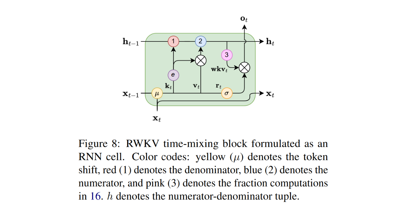
I am getting flashbacks about LSTM just from looking at it…
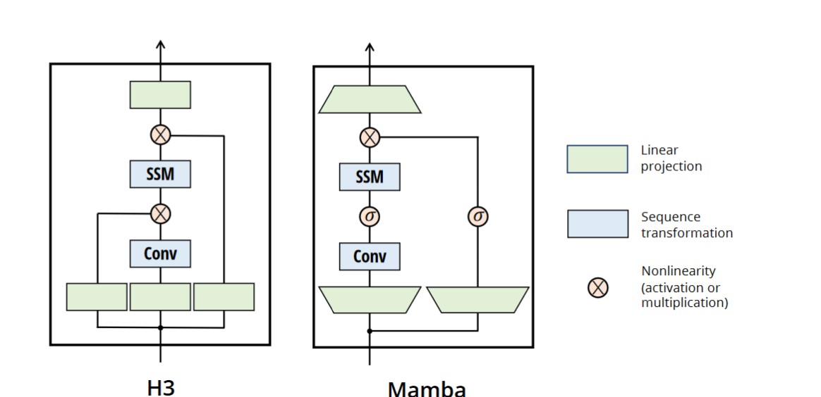
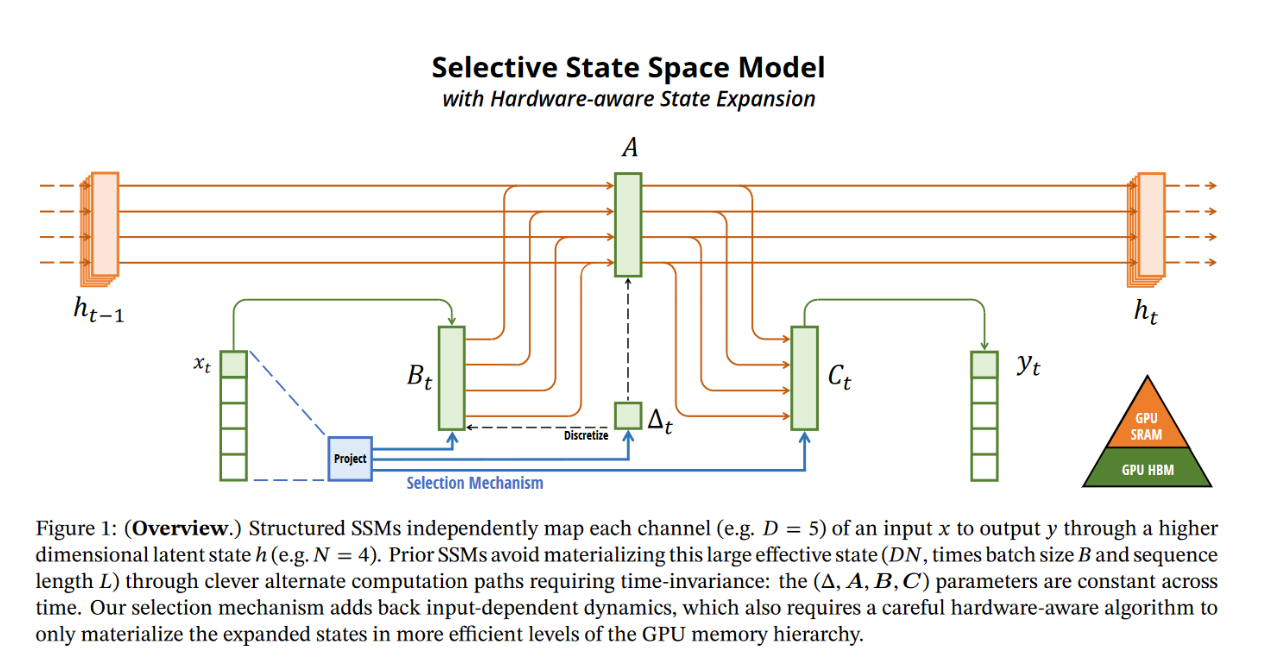
— Mamba makes the matrices B and C and the step size T in the state space model data-dependent.
If you want to see the formulas:

Note that T is always positive, which is logical, because it is the discretization step.
Let’s see what it means by examining the Euler approximation for the discretization:

When T → 0, this preserves the state and ignores the current input, while for larger T the current input gets more focus.
Modifying B and C to be selective also allows for additional control over whether to let the information about the input uₜ into the state xₜ and whether to let the state into the output yₜ.
By the way, if you look at the code of Mamba, you will find out that it does the following:

with elementwise multiplications.
The authors of Mamba also leveraged hardware (GPU) capabilities to make their architecture more efficient.
— Hawk (a subspecies of Griffin) suggests a Linear RNN model with the following recurrent layer architecture. Note that here we also have ⊙ (elementwise multiplication) instead of matrix multiplication:
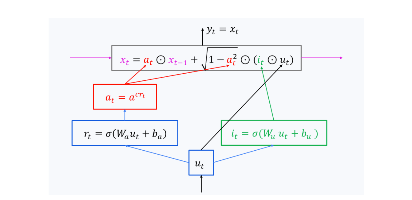
This mechanism, namely its

coefficients, allows for flexible control of how much info is retained from the history (xₜ) and how much is introduced from the new input uₜ. The authors claim that it is more convenient than Mamba’s (exp(TA), TB).
2.7. Hybrid architectures
Some authors note that using a mixture of recurrent blocks and multihead attention blocks improves quality while not undermining efficiency too much. Among interesting examples of hybrid architectures are the following:
- StripedHyena-Hessian-7B (SH 7B) is a hybrid of attention and state space models (more accurately, gated convolutions arranged in Hyena operators, but it is not very important right now).
- Griffin is alternating between two Hawk (recurrent) blocks followed by one residual block with local multi-query attention.
2.8. Results and impact
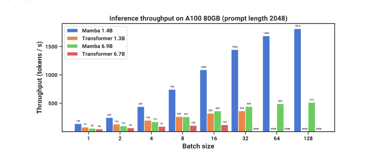
As you remember, we started with the problem of the inefficiency of transformers for long contexts. Inefficiency can come in the form of low inference throughput. In this context, RNN-based models perform well. Look at the results reported by Mamba.
You can also check out the results by Griffin:
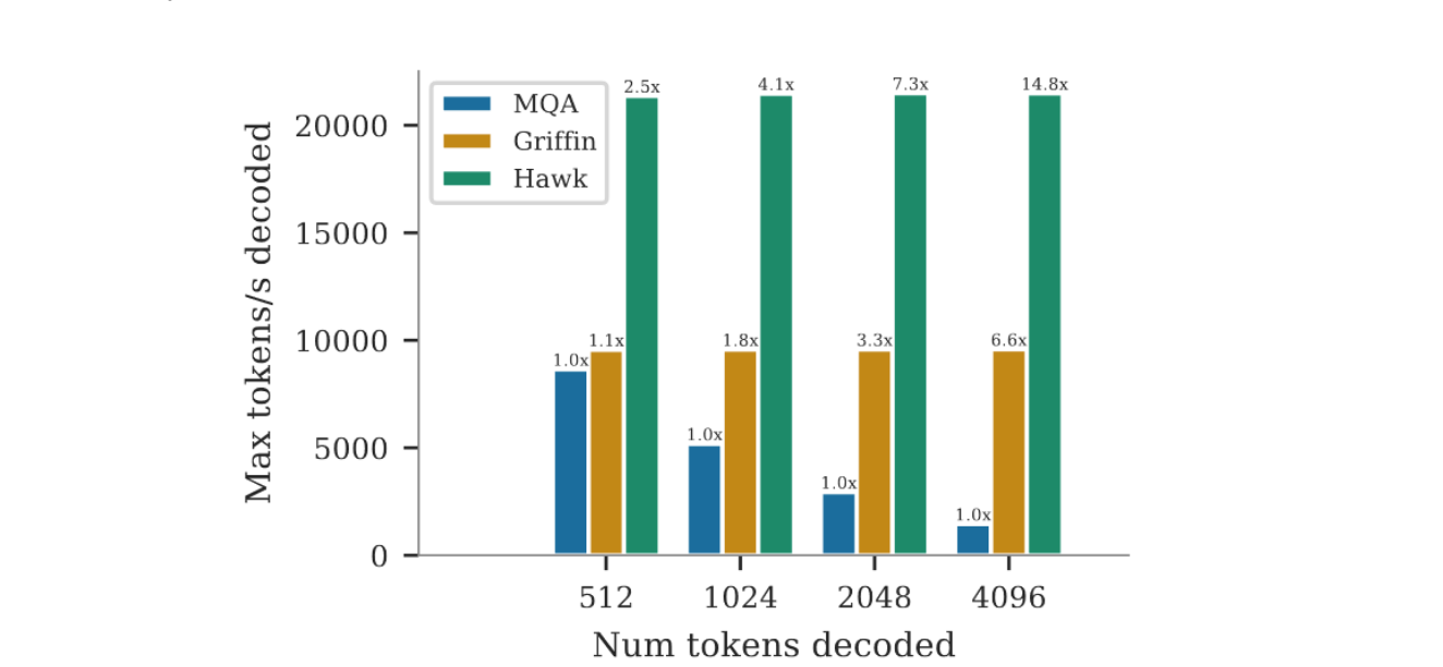
(b) Maximum throughput at 1B parameter scale.
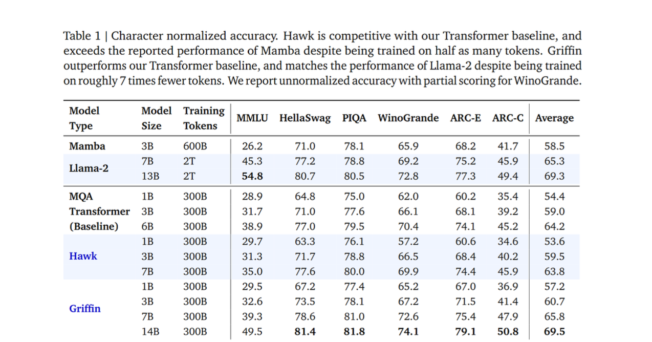
As for the quality, I would say that we still lack a full picture, but there are promising things like this table from the Griffin paper:
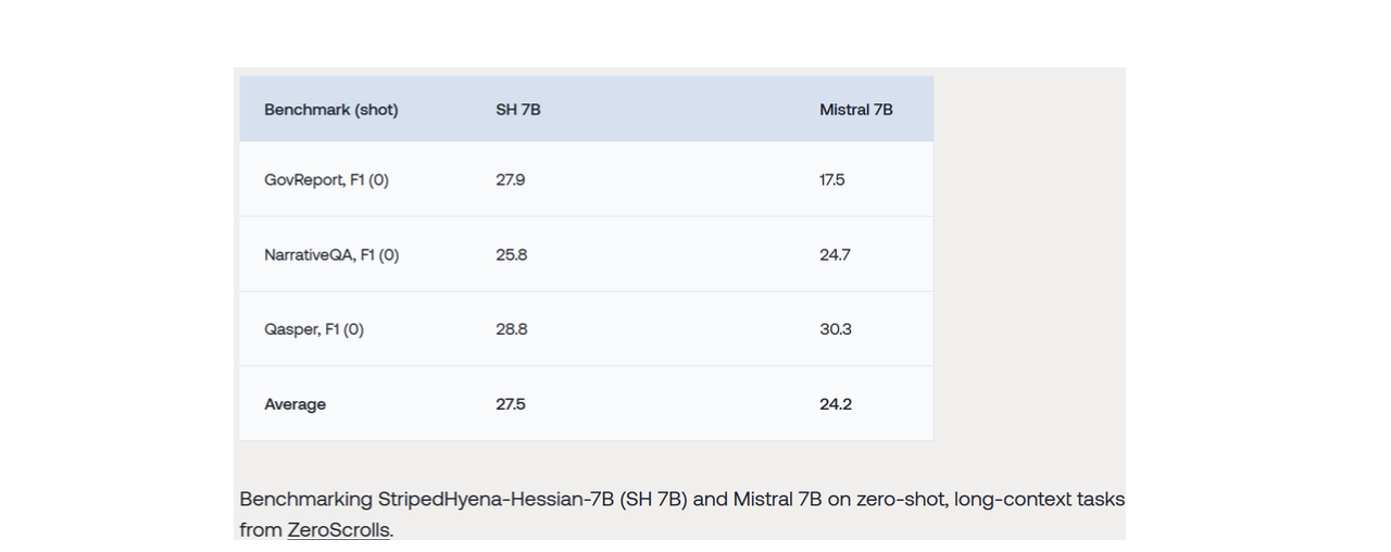
Benchmarks are also had been shared on Striped Hyena blog:
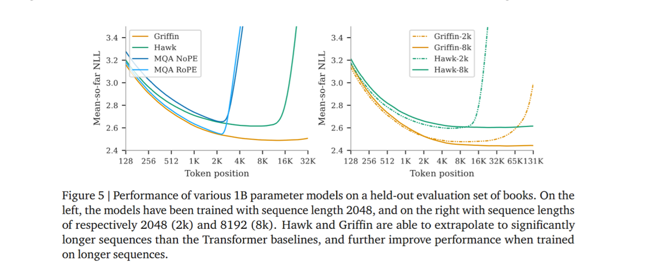
I would also add that these new models really are better at extrapolation to longer sequences. See, for example, these plots from the Griffin paper:
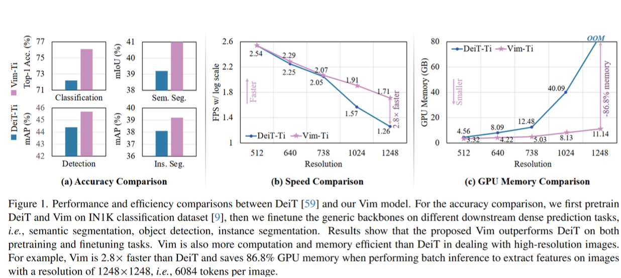
In the beginning of 2024, there was much enthusiasm about Mamba leading to several more Mamba-themed papers appearing. An example of them is Vision Mamba whose authors created a Mamba-based model for working with images that scales well with growing resolution (it is “vim” on the plots).
We do not observe wide adoption of Linear RNN-based or state space models into production yet. Partially, I think, this is due to healthy human conservatism. But it may well change in the future.
3. Paper reference
Relaxation of attention and Linear RNNs (non-state space models)
- An Attention Free Transformer — an attempt at relaxing quadratic complexity of a transformer.
- RWKV — block model with pure RNN time mixing blocks and recurrent MLP layers.
- Resurrecting Recurrent Neural Networks for Long Sequences — a very interesting theoretical analysis of Linear RNNs leading, in particular, to nice diagonal parametrization of A.
- Griffin.
State space models
- HiPPO — a new framework for understanding memory as compression capability.
- Combining Recurrent, Convolutional, and Continuous-time Models with Linear State-Space Layers — introduction of a Linear State-Space Layer (not for language modeling yet).
- S4 (see also this explanation) — strives to further increase the efficiency of state space layers through wise use of linear algebra (considering normal + low rank matrices for A).
- Hungry Hungry Hippos (H3) — dared to apply SSMs to language modeling tasks. Used block architecture that you have seen in the subsection 2.5. Proposed the new FlashConv mechanism that further improved the traditional FFT + pointwise multiply + inverse FFT scheme.
- Hyena Hierarchy — a long convolution sequence model (LCSM), highly influenced by SSMs.
- StripedHyena-7B — a model that leveraged all previous research (technically, it is a highly optimized hybrid of attention and gated convolutions arranged in Hyena operators).
- Mamba: Linear-Time Sequence Modeling with Selective State Spaces — no introduction needed at this point, I think.
- And finally, Vision Mamba.
I’ve initially prepared this material as part of the Practical Generative AI course by School of AI and Data Technologies. If you’re interested in studying LLMs and other generative models, their internal workings and applications, check out our program. In the meantime, I’ll continue publishing very technical articles on the Nebius AI blog, so stay tuned.
Explore Nebius AI